Home

Real Time Pathfinding Using Flow Fields Optimized with Navigation Meshes

Hello all! It’s been about three months since my last post, so I figured I would do one on my latest AI project: Flow Fields.

This post will begin with a brief overview of steering forces and flock systems, as these are crucial to understanding flow fields. Next, we will go into flow fields proper: how they are created for pathfinding and why you want to use them as opposed to say A-star pathfinding. Finally, I will detail how you can optimize flow fields with navigation meshes so that their generation is done quickly. Here is a simple video detailing what the result of all this looks likes:

(Click to watch video)

Before we get started, I wanted to touch on a couple of things. This entire post is detailing the flock system used in my project Alexander, which is basically an implementation of steering forces and flock behaviors in the Unity Engine. This is important because it will define some assumptions I am making about the systems we are dealing with: namely that the space you are working in is 2D and can be described by a grid of tiles. Despite this, you can extend this to 3D environments if you so desire.

Background – Steering Forces and Flock Systems

First, what exactly are “flow fields” and “steering forces” and “flock systems” for? As these names may imply, we are dealing with real time AI systems. Whether it be a game, simulation, or something else, the goal is to resolve paths through spaces with many agents running around.

So what is a “steering force”? They are vectors you apply to objects that move them. The important thing is that it does these movements smoothly. Let’s look at the graphic below:

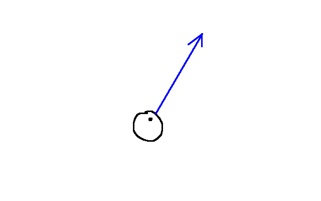
The blue arrow represents the velocity of the agent. Suppose now something happens in the simulation, and the agent want to go towards some goal:

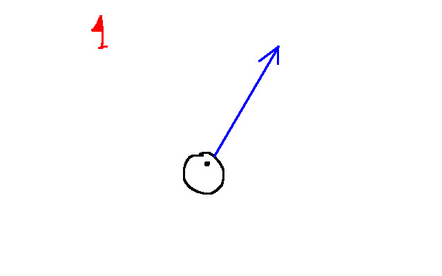
The red flag indicates the desired destination of the agent. Given this target, we can compute the desired velocity for the agent to move towards that goal:

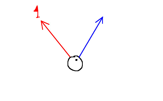
Now we have two velocities: one for the agent currently (indicated in blue) and one for what the agent wants to have (indicated in red). For each tick of your simulation, you can push the agent closer towards the desired velocity until it has it. In doing so, the agent will have a smooth transition from its current velocity to its desired one. With only a few lines of code, you can simulate birds, airplanes, horses, people moving, and so much more.

Another cool fact: steering forces can be combined! You could have one steering force that pushes you towards a goal, and some that push you away from hazards. The power of steering forces lies in its ability to create emergent behavior from simple rules:

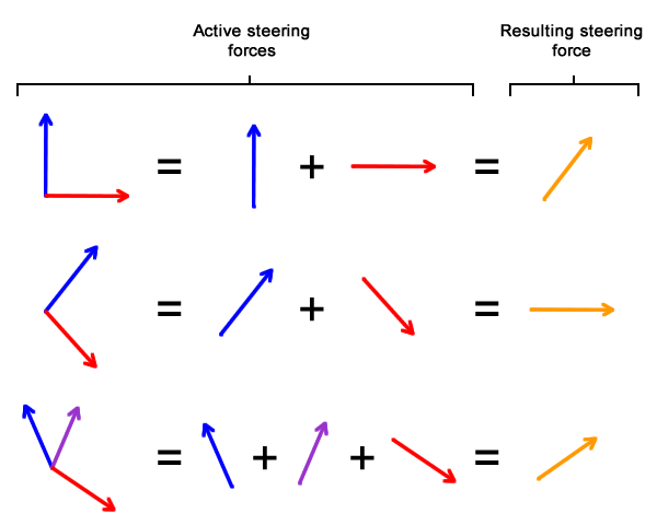Credit to Fernando Bevilacqua.

For the sake of this article, I won’t go into the math of them. You can find a million of such tutorials and articles online, and one of my favorite is a series by Fernando Bevilacqua.

So what are “flock systems”? They are an extension to basic steering forces. Steering forces give you the power to easily simulate individual agents. You can extend steering forces to simulate a flock of birds (hence the names “flock” or “boid” systems), thanks to the work of Craig Reynolds

Essentially, you begin with the idea that agents (from here on out called “boids”) are clustered into flocks. Then, using these flocks you can come up with new steering forces to govern groups of boids. The three main ones are:

• Cohesion: a steering force that encourages nearby boids to be closer to each other

• Separation: a steering force that, the larger its magnitude, encourages boids to maintain a distance from each other more

• Alignment: encourages boids to line up with other boids nearby in its flock

Images from Craig Reynolds

The article I posted above dives more deeply into the math of these, if you are interested in reading more about them. With a brief understanding of these concepts in mind, let us now dive into flow fields themselves.

Flow Fields

So we know how to move an individual boid, and we know how to move a flock of boids. This is great, but suppose you want to navigate a space with obstacles? We need some way to have our flocks navigate. It may be tempting to hit this with something like A-star, but there are runtime problems with this.

Consider a scenario where, for some reason, a member of the flock was separated from the rest of its group:

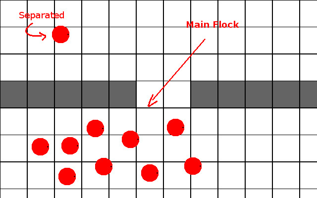
If we did a single A-star search for the entire flock, we run into an issue where this boid can’t navigate like the rest of the group because the path it would need is different. So we would probably have to do something like A-star on each of the individual boids. This would bring serious runtime problems in your simulation. Also, you would have to make sure your A-star search returns a list of steering forces that push your boids along the path. And if the path changes, you need to construct a new list.

The problems go on and on, but we can avoid all of them with Flow Fields.

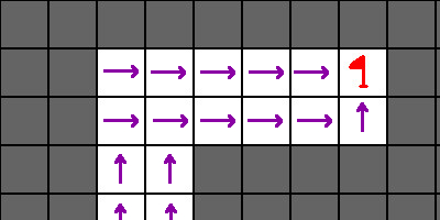
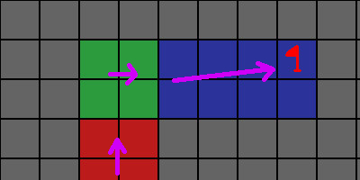
Suppose you have a tile grid of N rows and M columns. Then a flow field would be a 2D array of vectors with dimensions N rows and M columns. Given the entry (i, j), the corresponding vector would be a steering force that pushes you in the direction of the next tile. Ideally, if you follow these forces, they will eventually guide you towards a goal as depicted here:

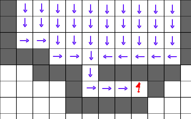
The dark grey tiles are walls. What makes flow fields attractive is the fact that they are easy to generate. Suppose you have a goal position that is the tile at (i, j). The algorithm for generating the flow field is as follows:

1. Create 2d array of vectors of size M by N (size of the tile grid). Call this T
	- Set each of these to some initial null value
2. Create a queue of unvisited positions Q
3. Add goal position to Q
4. While Q is not empty:
	-n = dequeue(Q)
	-For each neighbor w of n:
		- If T[w.row][w.col] is null:
			-T[w.row][w.col] = vector from w to n
			-Add w to Q

For a given flock, we need only one flow field to find the goal. This way, we can use the power of steering forces and flock behaviors while seamlessly adding pathfinding. Flow fields are not new: they were used in Supreme Commander 2 for pathfinding with groups of units.

Optimizing Flow Fields with a Navigation Mesh

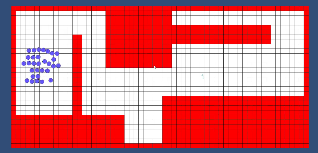
While flow fields are great, we can make them a little faster. If you’re space is really large, you are going to be search a lot of tiles. Is there some way we can make this faster? If you’re willing to eat some costs up front, then yes. What I mean is that we can spend some time at the start of the simulation computing a “navigation mesh”, which is a graph that groups walkable spaces together (the edges denoting which groups are adjacent). So in our space, groups of walkable areas would be groups of tiles. We do not group tiles arbitrarily – the next little example will hopefully give you an intuition for how we build our navigation mesh. Consider a level that looks like this:

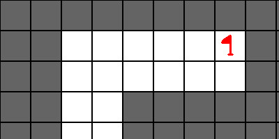
The red flag denotes the goal. Since we will compute a vector for all walkable tiles that can reach the goal, we don’t bother putting an agent/flock in this graphic. I will now show the same image overlaid with a navigation mesh:

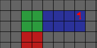
The walkable tiles are now colored according to the “navigation region” they are a part of. This partition was not arbitrary. All the regions are rectangles. This means each of these regions is convex. In other words: take any two points within the rectangle, and there is a line between them that does not intersect a wall. This is what we call a “direct line of sight”:

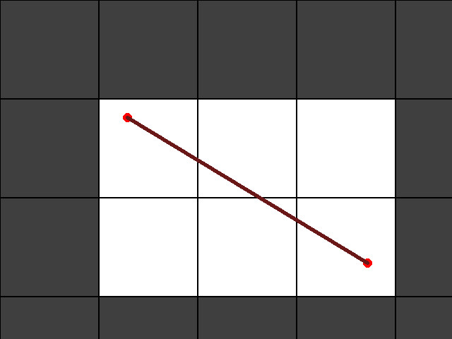
Yes, this is a contrived example, but it gets the point across. The white tiles are all in the same rectangular region, and the grey ones are walls. The red line is an example of “direct line of sight”. The top left tile and the bottom right tile have a line that goes directly between them that does not intersect any grey walls.

What is the implication of this? It means there is a steering force that will push you from one of these tiles straight to the next without hitting any walls. And this is true for all tiles in a single navigation region. Meaning: from any one tile in this region, there is a steering force to any other tile. Thus, you now have a guarantee that so long as your destination is in the same region, you will not bump into any walls.

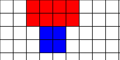
Furthermore, there is a relationship between the rectangular regions: If you are to combine a region with one that is directly adjacent to it, they will form a rectangle. This is important because it gives us another guarantee: there is a direct path of travel between any point in one region, and any point in an adjacent region:

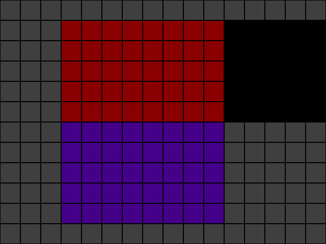
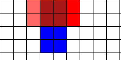
The red region and blue regions are both rectangles, so the property about line of sight among their constituent tiles holds. However, we can combine these two regions into a bigger one like so:

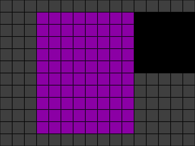
This means that every tile in both of these regions has a direct line of sight to any other tile in these regions. Witch means we can construct a steering force between any tile in these two regions.

Now what is the significance of these navigation regions? In the context of flow fields, we can say “what is true for one tile in this region is true for all tiles in this region”. Thus, we need only one steering force vector for each region. Going back to first example, if we wanted a flow field for it, we go from this:

to this:

Our search space goes from 16 walkable tiles to 3 regions.

There are two issues with this method: first is finding an algorithm to generate these navigation regions, which must be ran up front before the simulation begins.

The second is that you will only have an approximation to the most efficient path. There are some cases where the corresponding steering force for a particular tile will not point directly at the goal when it otherwise could have.

I personally found that such losses in accuracy in path solutions to be too miniscule to account for in a real time simulation like Alexander. There are ways to rectify this, but I will not detail them here.

Generating Navigation Meshes

I’d like to preface this by saying there are countless ways to create these navigation meshes (if you wanted, you could build them by hand too). As such, I am detailing the algorithm I designed for this. If you would like to see the source files in particular that implement this in Alexander, go here.

My algorithm has two phases to it:

• Generating the basic navigation regions such that they are all rectangle regions with no wall tiles in them.
• Splitting these navigation regions until every pair of adjacent regions is such that, if combined, form a larger rectangle that also has no wall tiles in it.

The first phase can be done in several different ways, so I will pass over how I did this part. It is the second part that, in my opinion, is far more salient.

It’s overall structure is:

1. found_split = true
2. while True:
	- found_split = false
	- scan each navigation region in navigation mesh.
		- If any region needs to be split into constituent regions:
			- split the region
			- place results in navigation mesh
			- found_split = true
	- if found_split is false:
		- break

Essentially, we continue to “split” these regions until it is no longer possible. What does it mean to “split”? Suppose I have two adjacent regions that are as follows:

I need to pick one of these pieces and break it in either two or three pieces, perhaps as follows:

Hopefully you can see now the regions are split such that they fulfill the guarantees we wanted with our navigation regions: every navigation region is a rectangle, and each region could be combined with any one of its neighbors to form a bigger rectangle. By having these constraints we ensure that each tile within a region has a direct line of sight to each tile in an adjacent region. Thanks to this, we can do flow field generation on entire regions instead of one tile at a time. This saves on both space and run costs.

And that’s it for this post. I hope you found this useful. Please do checkout my project Alexander if you want to see this system in action.

Home