Liam Wynn
This is my site. Here, I make neato projects and blog posts.
Implementing a Ray Caster Part 1: Basic Wall Rendering
Hey all! This is a long overdue series, but I’m finally getting around to it. I will be detailing my implementation of the ray casting algorithm used in the classic Wolfenstein 3D to render its environments. I implemented it as a part of my final project for CS 410p: Full Stack Web Development, taught by Brian Ginsburg. It was a purely front-end application. As such, I’ll post my results either on its own Github.io page, or somewhere on here. In the meantime, you can check out the levels I did for it here.
Also, I want to give credit to Permadi. It was thanks to him that I could implement what I have here, so please please please check out his work.
Section 1: The Setup
With that little introduction out of the way, let’s get to it. Today’s post is getting an idea about the underlying mathematics before we dive into implementation details. But don’t worry! We just need some high school level geometry. If you’re comfortable with that, you should be okay.
First and foremost, we’re going to make a couple of assumptions about what our worlds look like, and how they behave. I think this really awesome graphic more-or-less summarizes the parameters of our worlds:
As the graphic implies, our worlds are actually 2D! Most of the magic is done on a single plane. I’ll explain how we translate 2D computations into 3D environments. Also, as the graphic shows, our worlds are not just top-down and two dimensional. The world is a series of tiles. In more advanced versions of ray casting, you can variations in the height of walls, sprites (as I call them, “things”), and so on. But I kept it simple. I assume that every wall is perpendicular to other walls, and equal in width, height, and depth.
Basically, the assumptions we make are as follows:
- The underlying representation of worlds is a 2D tile grid.
- The squares of this grid are either a walkable area or a wall.
- All walls are perpendicular to each other.
- All walls are equal in height.
By making these assumptions, we drastically reduce the complexity of rendering.
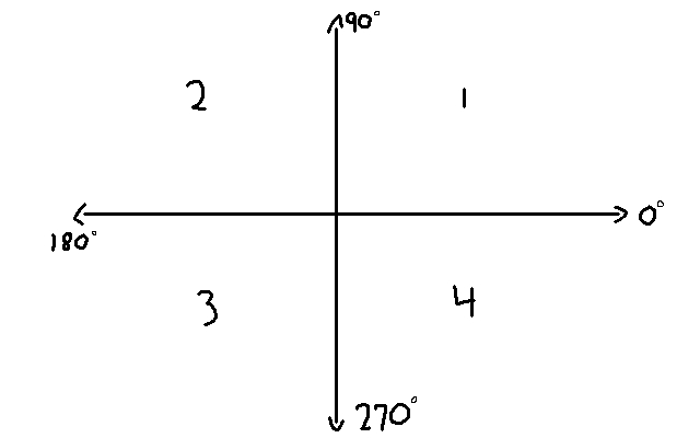
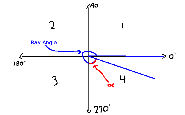
One quick side note: this graphic shows our coordinate system. I mentioned it earlier, but let’s make sure it’s fleshed out. Note that the XY plane is viewed from the top-down. So the z axis points upwards in our 3D rendering.
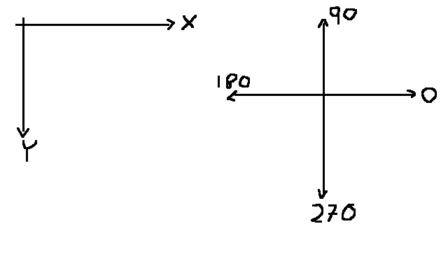
On the left hand side is the XY-Plane. Note that Y is pointing downward, which is an artifact of how graphics are typically rendered. The right hand side is the orientation of a unit circle. Note that the units, while technically unspecified in the image (it was quickly done), are in degrees. This is important for later, when we explore optimization techniques.
Okay so we’re ready to start firing rays out and rendering worlds, right? Well not quite. There’s a couple of parameters we need to establish first. I will give you the parameters I used in my implementation:
- The screen width and height, which we’ll call the “Projection Plane”, as a width of 320 pixels and a height of 200 pixels.
- The units we deal in for the size of walls, floors, ceilings, and sprites is always 64 pixels by 64 pixels.
- The field of view for the player is 60 degrees.
- The player’s height is 32 pixels.
Let’s see some graphics of these so far:
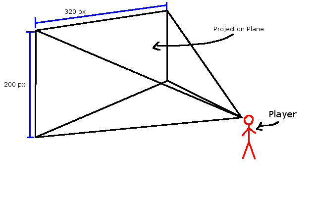
So here is what our screen/projection plane looks like in the 3D world. Interestingly, my graphic implies that there is a distance between the player and the projection plane. Not only is this true, but it’s important that we know this distance later on down the road.
Okay so why do we care about these values? Well the field of view specifies what we can see in the 3D world. But we need to be able to render that to a screen size of 320 pixels by 200 pixels. Also, by knowing the size of everything we deal with (and the units too), we can simplify some of the math. With these values, we can compute two things: the angle between each ray, and the distance of the projection plane to the player. Let’s explore these:
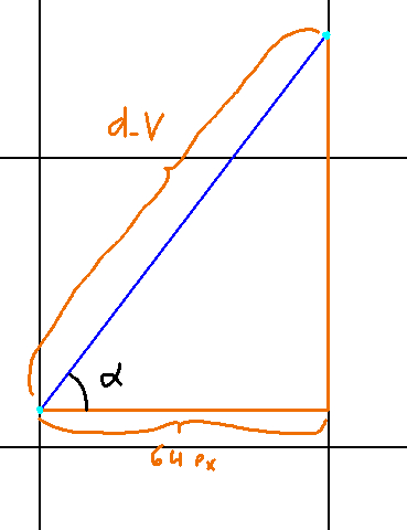
First, we know the field of view, which is 60 degrees in our case. Our projection plane width (aka: screen width) is 320 pixels. So we can compute the angle between each column of pixels as 60 / 320 = 0.1875 degrees per column of pixels. Next, let’s examine the graphic below:
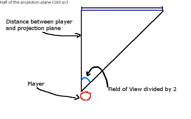
To compute the distance between the player and projection plane, we can use good ol’ Soh Cah Toa. In this case, we’d use Toa: The tangent of the field of view divided by two equals the opposite leg to our angle (the projection plane / 2) divided by the adjacent leg (the distance between the player and projection plane). In condensed math notation, that becomes: tan(30) = 160 / dist_to_proj. Solving for dist_to_proj, we get dist_to_proj = 160 / tan(30) = about 277 pixels. We’ll just round down to keep our computations simpler. I should note that in my implementation, I wanted to explore optimization tricks and was thus willing to give up precision.
So a quick summary of what we now have:
- Projection Plane = 320 pixels in width by 200 pixels in height.
- Field of View = 60 degrees
- The size of everything is 64 pixels: So walls are 64 pixels by 64 pixels, sprites are also 64 x 64 pixels.
- Player height is 32 pixels.
- Angle between columns of projection plane = 60 degrees / 320 pixels = 0.1875 degrees per column of pixels.
- Distance to projection plane = (projection_plane.width / 2) / tan(fov / 2) = 160 / tan(30) = about 277 pixels.
With all of this, we are now ready to take on the core of the algorithm: rendering walls.
Section 2: Wall Rendering – Deciding What to Render
Let’s begin by thinking about how we rendering what we see? This is where the “ray” part in raycasting comes into play. The general algorithm looks like this:
For each column of pixels in our screen:
	-Fire a ray that starts from the player, and travels along the angle that corresponds to our current column.
	-If this ray hits a part of a wall, render that part of the wall.
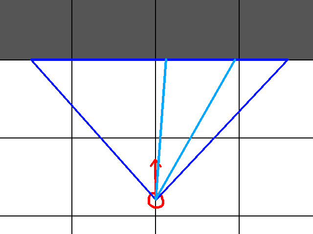
Well that’s a curiously tiny algorithm. However, it is a bit deceptive. Angle that corresponds to our current column? Rays? Rays hitting walls? There’s a lot at play here. So let’s try to visualize this. I think the graphic below does a pretty good job
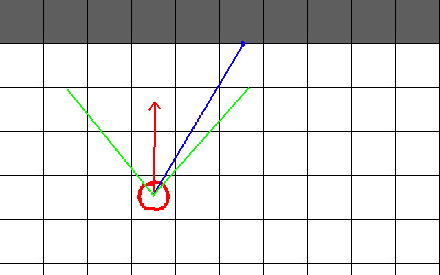
Here is a top down view of our set up. The white tiles are walkable areas (ie: not walls). The dark grey tiles represent walls. The red circle is the player. The red arrow extending from the player is his rotation. The green lines represent the bounds of the field of view. Finally, the blue line represents the ray we are interested in. There’s a lot of things we need to note from this graphic:
- The angle between each of those green lines is our field of view (in this case, 60)
- From the left most green line to the right most, there are 320 rays we will compute, since that is the number of columns in our projection plane.
- The red arrow splits our field of view in half. So that is, the angle between the red arrow and the leftmost green arrow is 30 degrees. Similarly, the angle between the red arrow and the rightmost green arrow is also 30 degrees.
- Therefore, suppose our red arrow, the player’s rotation, is theta. Then the angle of the leftmost green line is theta - (field of view / 2) = theta - 30. Likewise, the angle of the rightmost green line is theta + (field of view / 2) = theta = 30.
So now we can figure out the “angle that corresponds to our current column”:
- Suppose the leftmost column of our projection plane is Column 0. Then the rightmost would be Column 319 (therefore, there are 320 columns).
Now we can rewrite our algorithm to be a little more descriptive:
curr_ray_angle = theta - 30
For each column of pixels in our projection plane:
	-Fire a ray that starts from the player and travels along the angle curr_ray_angle
	-If this hits a part of a wall, render that part of the wall.
	-curr_ray_angle += 0.1875 degrees
So wait, why do we add 0.1875 degrees every iteration? Remember, we have 320 columns of pixels in our screen/projection plane. We also have a field of view of 60 degrees. So to relate these things, we divide 60 degrees amongst 320 columns to get 60 degrees / 320 columns = 0.1875 degrees per column. Hence, to go from Column n to Column n + 1, we must add 0.1875 degrees.
Okay so now that we more concretely understand the relationship between the width of the projection plane, the field of view, and the angle of each ray we cast, let’s figure our how to actually detect a wall hit. We’re going to do so by starting with a naive algorithm, and then use a little bit of trigonometry to design something better.
We know the angle each ray tavels at, and we know where it starts. Naturally, we might think the best or only solution is the one below:
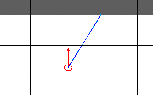
In this system, our ray travels a tiny bit and checks to see if a wall was hit. If not, we move the ray a little bit more. The deep blue line is our ray in this graphic, and the light blue dots are where we check if a wall was hit. The pseudocode for this might look as follows:
movement_magnitude = 5
while the current ray has not hit a wall:
	current ray x += cos(ray_angle) * movement_magnitude
	current ray y += sin(ray_angle) * movement_magnitude
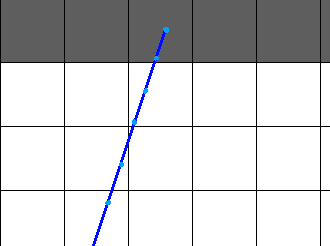
The problem with this algorithm is that we need to tune the movement_magnitude to find a “Goldilocks value”. If movement_magnitude is too small, we will perform too many computations potentially. If it’s too large, we may skip over walls. Furthermore, it’s highly unlikely that you’ll actually hit the side of a wall, as the graphic shows. More than likely, you’ll hit somewhere in the interior like this:
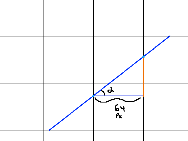
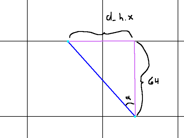
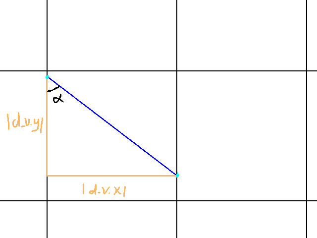
There are ways to account for this, but it’ll very likely become more trouble than its worth. Instead, we can take advantage of the tile system we’re working with. Since our world is a tile grid, we know that the distance between say two horizontal gridlines is the same (in this case, 64 pixels). That is, to go from the one horizontal gridline to the next, I must travel 64 degrees upward or downward. The graphic below demonstrates this:
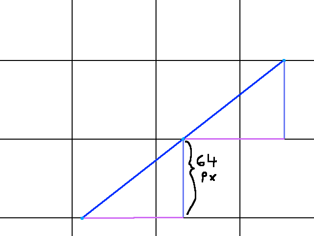
In fact, our graphic details a lot more than just the distance between horizontal gridlines. The angle there, alpha, is the angle of the ray (adjusted to its quadrant, more on that in a bit). Notice how a triangle forms between the segment of the ray (blue), the distance between horizontal gridlines (purple), and the distance travelled along the x axis to get from one light blue dot to the next (pink). What’s more, this triangular relationship repeats between tiles. At no point in the ray’s lifetime will this relationship change. So any information we extract from this pattern will remain constant (until the ray hits a wall). A similar pattern holds for examining what happens as the ray is going between vertical gridlines, as shown below:
What is different is now we know that to go from one vertical gridline to the next, we must travel 64 pixels along the X axis. The value we don’t know is the orange line segment, which is the y-axis change as the ray travels between two vertical gridlines.
As you’re probably guessing, we are going to solve for those pink and orange line segments, right? Of course. But let’s get some motivation for how this will help us. Recall the naive algorithm we had. As I mentioned, it could either be too many computations if your ray’s movement magnitude was too small, or entirely miss walls if it’s too large. By using the relationships we have above about gridlines, we can guarantee that we hit walls (provided the level has no leaks in it), and significantly reduce the number of computations than our other algorithm. For comparison, here is our old algorithm:
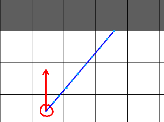
And here is a visualization of what our new algorithm will do:
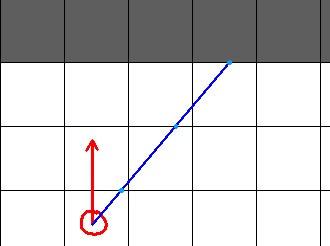
And, finally, if we go with the change in vertical gridlines instead of horizontal ones:

There are several things to note. Clearly, we see that the number of light blue dots is significantly reduced. I will say, in fairness, that this may not be the case, depending on the movement magnitude you choose. Again though, reducing the computations implies you’ve increased the magnitude, which means that you run the risk of missing walls you should not have. This new method, on the other hand, garantees that we hit the appropriate wall.
Second, we see that choosing to look at vertical or horizontal gridline has a huge impact on where we hit the part of the wall we want to render. As such, our algorithm will require us to look at the blue dots that jump between vertical gridlines and horizontal gridlines.
I think it would be instructive if we saw a broad overview of the algorithm before we get into it. In essence, it looks like the following:
let c_h be the point where our ray would intersect the closest horizontal gridline.
let c_v be the point where our ray would intersect the closest vertical gridline.

let d_h be the vector describing how much we move c_h to get to the next horizontal gridline.
let d_v be the vector describing how much we move c_v to get to the next vertical gridline.

while c_h is not intersecting a wall or out of bounds:
	c_h += d_h

while c_v is not intersecting a wall or out of bounds:
	c_v += d_v

if both c_h and c_v interesct a wall:
	return the one closest to the player.
if c_h is out of bounds:
	return c_v
if c_v is out of bounds:
	return c_h
if both c_h and c_v are out of bounds:
	return an error vector
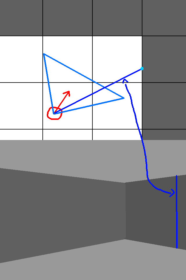
And here is a visualization of the algorithm:
In the first frame, we see where c_h is initially. The second frame shows where d_h comes from. The second light blue dot is c_h + d_h. Since it hits a wall (the dark grey tile), we stop that point in the algorithm, and start to look at c_v. First we see where c_v starts, in frame 3. Then the interesting thing is that d_v is a vector that goes past the bounds of the image. Hence, when we add d_v to c_v, we cannot see where the next light blue dot is. In this scenario, c_v is outside the bounds of the level. Hence, we go with c_h as where our ray hit.
It is possible for c_h or c_v to be outside the bounds of the world and not render anything. In my implementation, this happens frequently. I simply terminate the rendering algorithm for that ray. If your implementation doesn’t do optimizations that compromise precision, you will likely only encounter weird edge cases where rendering fails.
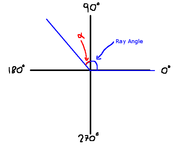
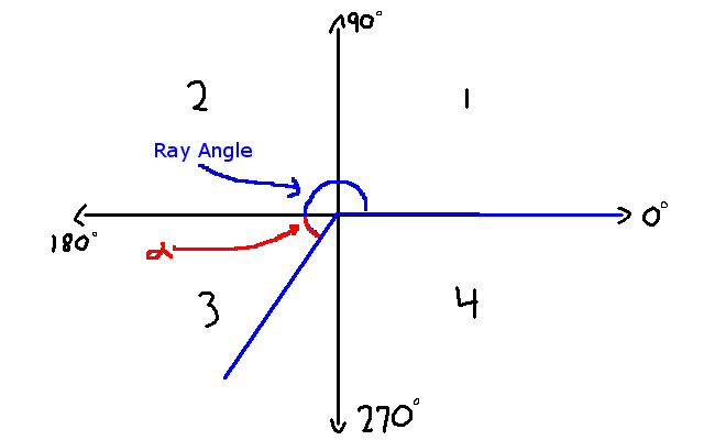
Now I think we know enough about the algorithm to see the mathematics of it. To begin computing c_h, c_v, d_h, and d_v, we must first figure our what quadrant our ray’s angle is in. Why is that? Well we have to adjust the angle depending on the quadrant. I’ll show you what that looks like as we explore each case. For now, here is a graphic showing our four quadrants:
Now, let us explore each of these cases:
Quadrant 1 (0 < Ray Angle < 90)
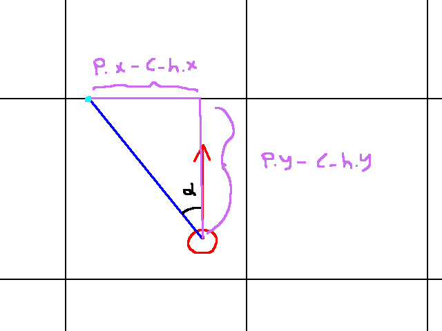
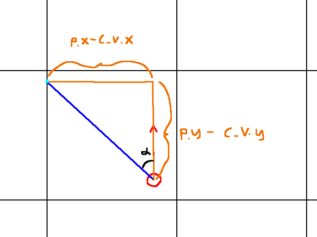
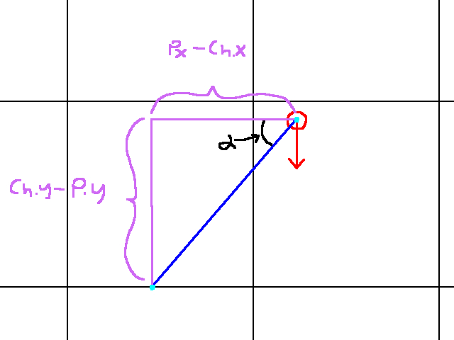
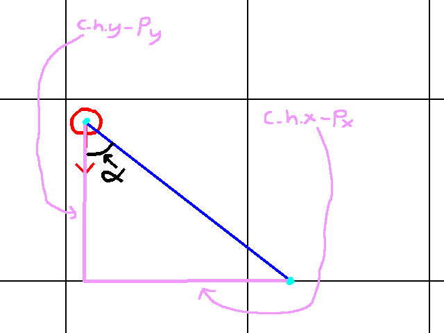
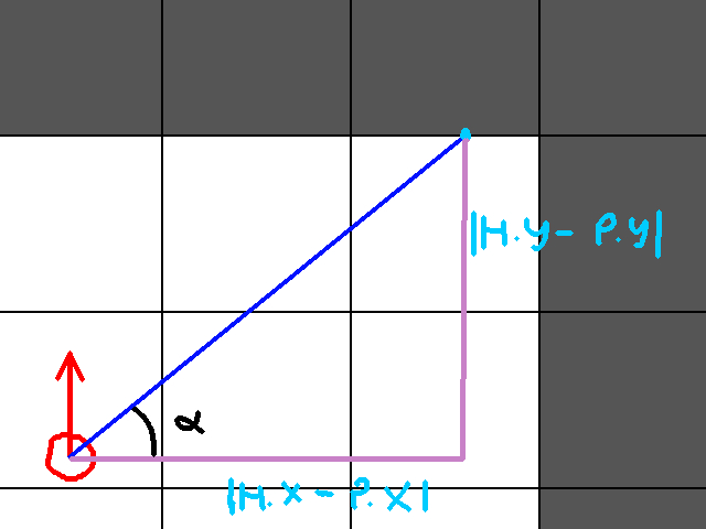
In this case, we don’t have to worry about adjusting our angle in anway. Let’s go ahead and figure out c_h and d_h. As I said before, finding c_h means finidng the point at which our ray intersects the closest horizontal gridline. A graphic of this details this:
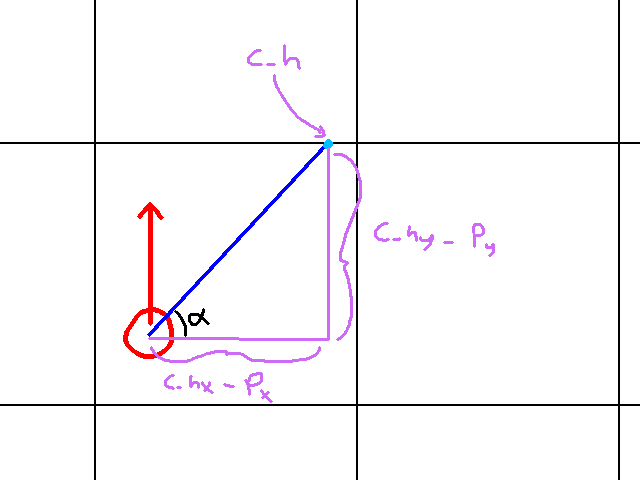
What’s cool about this graphic is it visualizes the relationship between the player’s position, the ray angle, and c_h. Since we’re in quadrant 1 in this case, we know that c_h has a greater y value and a greater x value than the player. Hence, c_h.y - player.y > 0 and c_h.x - player.x > 0. Unfortunately, Soh Cah Toa won’t help us a lot in this case. To find c_h.y we need c_h.x and vice versa.
However, we do know that c_h is on a horizontal gridline somewhere. And it’s not just any horizontal gridline: it’s the one directly above the player! And it makes sense: our ray’s angle is in quadrant 1 (relative to the player), so it has to travel in a positive x and y direction. To compute the y component of c_h, we do the following:
c_h.y = (floor(player_pos.y / 64) * 64) - 1
So first, we divide the player’s y position by 64 and floor the result. Remember: everything is 64 pixels in size. So that means our player’s world position divided by 64 gives us the current tile he is in. We have to floor it because if the player is likely in the middle of the tile. Thus, his position divided by 64 might give us something like 5.1484. This would tell us he is in tile 5, but about 14.84% of the way into it, so to speak. If you’re doing all this math with integers, then the floor operation is unnecessary since you will get a rounded down result by default. Then we multiply the result by 64. So again, if the player’s y position divided by 64 was 5.1484, then we floor it we get 5, and then multiplying by 64 once again we get 320. This would give us the global position of the gridline. As a safety precausion, we subtract 1. Remember: our coordinate system has it so that going upwards decreases the y value. By substracting 1, it puts us in the tile above our player. Without it, we might be one pixel off from hitting a wall. However, our system would ignore the wall we should have hit.
Now that we have c_h.y, we can find c_h.x. At this point, it’s okay to use Soh Cah Toa. We want the adjacent leg to the alpha in the graphic above. And we have the opposite leg. Hence we will go with Toa in this case. That is:
Tan(alpha) = opposite leg / adjacent leg.
We can replace “opposte leg” and “adjacent leg” with more informatvie values. Giving us:
Tan(alpha) = (c_h.y - player.y) / (c_h.x - player.x)
And now with a little bit of algebra we can say:
c_h.x - player.x = (c_h.y - player.y) / Tan(alpha)
Finally, we add player.x to both sides and we get:
c_h.x = ((c_h.y - player.y) / Tan(alpha)) + player.x
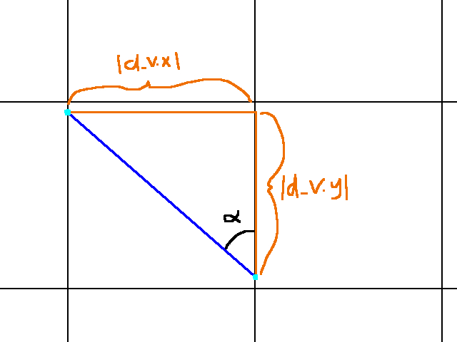
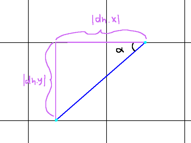
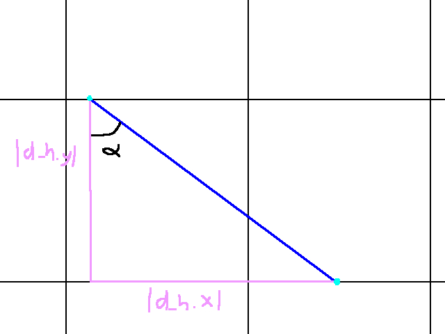
And there we have it! We’ve computed c_h for quadrant 1 ray angles. Now let us go ahead and find d_h. Recall that d_h describes the vector between one horizontal gridline to the next. Graphically, that would be this:
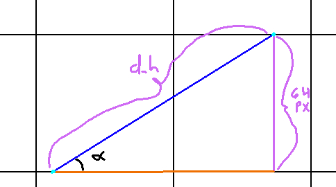
Finding d_h in quadrant 1 is a much more straightforward problem. We know alpha (our ray angle), and we know that to go from one horizontal gridline to the next, we must move 64 pixels in the y-axis. Actually, more specifically, we need to travel -64 pixels in the y-axis (since traveling upwards is going negative in our coordinate system). But for computing d_h.x, we will use all positive values. Once again, we employ Toa here:
Tan(alpha) = opposite / adjacent
Equivalently:
Tan(alpha) = 64 / d_h.x
and hence we get:
d_h.x = 64 / Tan(alpha)
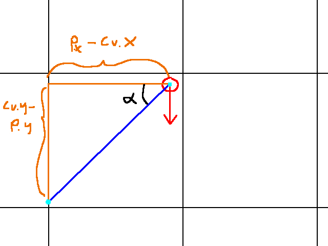
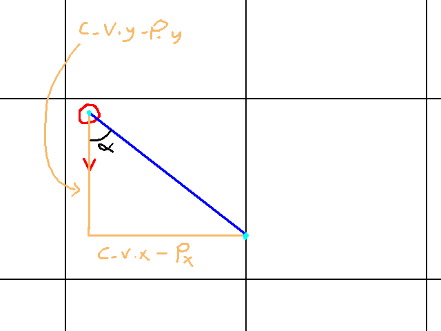
Great! We have c_h and d_h in quadrant 1. Now we have to repeat the process for c_v and d_v. Once more, let’s see a graphic to visualize c_v:
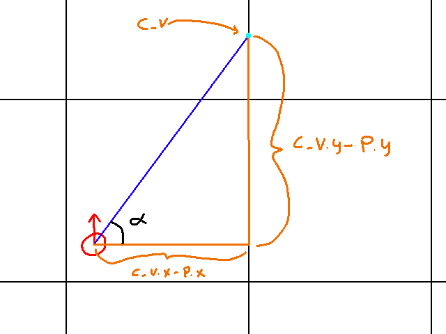
Like c_h, we’re a bit stuck because to find c_v.y we need c_v.x and vice versa. Like before, we exploit knowledge about c_v to find one of its component values, then use that to find the other. In this case, we know c_v.x is on a vertical gridline. To go from one vertical gridline to the next, we need to travel 64 pixels in the x axis. As such, we can compute c_v.x as follows:
c_v.x = (floor(player.x / 64) * 64) + 64.
Essentially, we find the tile number the player is on by computing floor(player.x / 64). Then we multiply this by 64 to get the vertical gridline that is 64 pxiels to the left of the vertical gridline c_v is on. That’s why we add 64 pixels to get c_v.x.
To get c_v.y we use Toa once more. That is:
Tan(alpha) = (c_v.y - player.y) / (c_v.x - player.x)
This implies:
c_v.y - player.y = Tan(alpha)(c_v.x - player.x)
And thus:
c_v.y = Tan(alpha)(c_v.x - player.x) + player.y
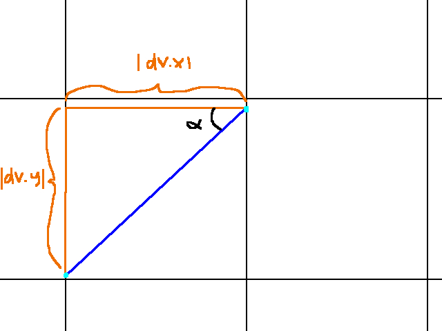
Now once we’ve got c_v, we just need d_v. To visualize this, our problem looks like the following:
This time, we know the distance between two vertical gridlines: 64 pixels. What we do not know is the y value of d_v. However, like everything else, this is just an application of Toa. That is:
Tan(alpha) = d_v.y / d_v.x
Thus:
d_v.y = -Tan(alpha)(d_v.x)
Whoah wait a minute, where did the negative sign come from? Remember, to travel up in the y-axis, we decrease our value. The y-axis is flipped from what you were taught in school. This is an artifact of rendering graphics to a screen, if I recall, although I don’t entirely know the history of it.
Anyways, we’ve computed all of the components for quadrant 1. Now we just do everything again from quadrants 2, 3, and 4. Before we do those cases. I want to summarize everything so far:
Computations for Quadrant 1
- c_h.x = ((c_h.y - player.y) / Tan(alpha)) + player.x
- c_h.y = c_h.y = (floor(player_pos.y / 64) * 64) - 1
- d_h.x = 64 / Tan(alpha)
- d_h.y = -64 (Since we travel in the negative direction along the y-axis)
- c_v.x = (floor(player.x / 64) * 64) + 64
- c_v.y = Tan(alpha)(c_v.x - player.x) + player.y
- d_v.x = 64
- d_v.y = -Tan(alpha)(d_v.x)
Quadrant 2 (91 < Ray Angle < 179)
In this scenario, we are in the top left quadrant. This means both the x and y direction of our ray angle is going to be negative. But as I mentioned earlier, our ray angle needs to be adjusted. If you look at alpha in quadrant 2, you notice that it’s an acute angle. That is, its less than 90. However, if its in quadrant 2, its going to be greater than 90. Let me show you a graphic comparing the adjusted angle alpha to the actual ray angle:
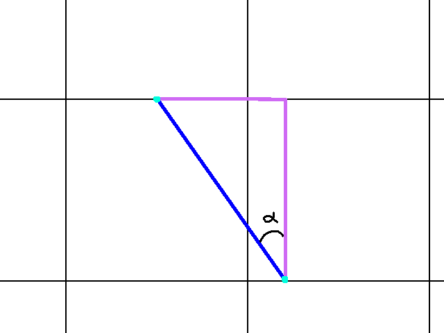
So this looks similar to what our problem in quadrant 1 looked like. However, the ray angle we have to work with looks something like:
For comparison, I showed alpha in relation to the ray angle. The angle alpha is the part of the ray angle that is entirely within our desired quadrant. Since the rest of the ray angle is in quadrant 1, we subtract 90. That is:
alpha = ray angle - 90.
And now we may proceed to use alpha in the same fashion we did when dealing with the quadrant 1 case.
We’ll begin with finding c_h. Recall that c_h is the point where the ray first intersects a horizontal gridline. In quadrant 2, that is as follows:
In this case, our ray travels in the negative x and y direction. The strategy for finding c_h will be to find c_h.y first, then use Toa to get c_h.x. The computation for c_h.y is the following:
c_h.y = (floor(player.y / 64) * 64) - 1
First, we divide the player’s y position by 64 and floor the result. This tells us the row of the tile grid the player is standing on. When we multiply it by 64 again, this gives us the global position of the horizontal gridline c_h is on. Subtracting 1 ensures the value is in the tile above the player. That way, when we do the computation, we are guaranteed to intersect a wall should there be one above us.
Next, to get c_h.x we do the following computation:
c_h.x = Tan(alpha) * (player.y - c_h.y)
First, we know that by Toa, the following is true:
Tan(alpha) = (player.x - c_h.x) / (player.y - c_h.y)
And then some rudimentary algebra gives us c_h.x, which for brevity’s sake I will not show here as I did previously.
With c_h resolved, we must now solve for d_h. This is the vector the ray must travel to get from one horizontal gridline to the next. Visually, that is as follows:
In this case, d_h.y is already taken care of for us. Since we travel in the negative y direction to get to the next horizontal gridline, d_h.y is:
d_h.y = -64
So to get d_h.x, we must once more employ Toa. The relationship is the following:
Tan(alpha) = abs(d_h.x) / abs(d_h.y) = abs(d_h.x) / 64
Than solving for abs(d_h.x) gives us:
abs(d_h.x) = 64 * Tan(alpha)
What I should mention is that the legs of our triangles are assumed to be positive, since they represent magnitude values along the x and y axes. Since d_h.x (and d_h.y) is negative, the absolute value gives us:
-d_h.x = 64 * Tan(alpha)
Thus, we our final result will be
d_h.x = -64 * Tan(alpha)
Next comes c_v. Visually this is what we are looking at:
We will begin by finding c_v.x. The computation is:
c_v.x = (floor(player.x / 64) * 64) - 1
In this case, we divide the player’s x value by 64 and floor the result. This tells us the tile column the player is on. We multiply this by 64 to get the global x value of the vertical gridline. Like previous cases, subtracting 1 ensures we are in the tile adjacent to us. From this, it’s easy to see how c_v.y is handled. we can solve for it by employing Toa. That is, Tan(alpha) = (player.x - c_v.x) / (player.y - c_v.y). Then some algebra gives us:
c_v.y = player.y - ((player.x - c_v.x)/ Tan(alpha))
Finally, we must find d_v. Our graphic for this is as follows:
Upfront we’re given d_v.x. Since we travel in the negative x direction, the value is:
d_v.x = -64
Then solving for d_v.y is a matter of applying Toa here. The result is:
abs(d_v.y) = abs(d_v.x) / Tan(alpha) = 64 / Tan(alpha)
Since d_v.y is negative, the absolute value gives us:
-d_v.y = 64 / Tan(alpha)
Thus, our final operation is to negate both sides:
d_v.y = -64 / Tan(alpha)
And there we have it! Quadrant 2 is solved. I will post a summary of all the necessary computations, then we shall move on to Quandrant 3.
Computations for Quadrant 2
- alpha = ray angle - 90
- c_h.y = (floor(player.y / 64) * 64) - 1
- c_h.x = Tan(alpha) * (player.y - c_h.y)
- d_h.y = -64 (Since we travel in the negative direction along the y-axis)
- d_h.x = -64 * Tan(alpha)
- c_v.x = (floor(player.x / 64) * 64) - 1
- c_v.y = player.y - ((player.x - c_v.x)/ Tan(alpha))
- d_v.x = -64
- d_v.y = -64 / Tan(alpha)
Quadrant 3 (181 < Ray Angle < 269)
Up until now, our y value has always been negative. With quadrants 3 and 4, this changes. As such, I will have to warn you, our graphics will look a bit different. Like quadrant 2, we need to adjust our ray angle to be something workable. Visually, we can represent the difference between the ray angle and alpha like so:
So computing alpha would be:
alpha = ray_angle - 180
We’re now ready to solve the rest of quadrant 3. As per usual, we’ll start with c_h. Our problem graphically is the following:
As you can see, the player is now looking downwards. However, this doesn’t change our math significantly. Since c_h is on a horizontal gridline, we’ll solve for c_h.y first. The computation is:
c_h.y = (floor(player.y / 64) * 64) + 64
First we divide the player’s y position by 64 and floor the result. This tells us the tile row he is on. Then we “undo” this by multiplying by 64. However, by flooring, we lost where exactly on the tile he was. As such, this gives us the position of the y position of the horizontal gridline above the player. Hence, by adding 64 this gives the position of the horizontal gridline below the player, which is the y position of c_h.
Next we can apply Toa to get:
Tan(alpha) = (c_h.y - player.y) / (player.x - c_h.x)
Then some simple algebra will yield:
c_h.x = player.x - (c_h.y - player.y) / Tan(alpha)
Very good. Next let’s go and find d_h. Once more, a visualization:
Notice that to go from one horizontal gridline to the next, we travel 64 units along the y axis. Hence:
abs(d_h.y) = 64.
Now since we’re traveling in the positive y direction:
d_h.y = 64.
Next for d_h.x, we note that:
Tan(alpha) = abs(d_h.y) / abs(d_h.x)
Thus:
abs(d_h.x) = abs(d_h.y) / Tan(alpha)
Now, since we are going in the negative x direction, our result will be:
d_h.x = -64 / Tan(alpha)
So we’re half way done with Quandrant 3. All that’s left is c_v and d_v. For c_v our problem looks like:
Since c_v.x is the vertical gridline to the left of the player, we’ll find it with:
c_v.x = (floor(player.x / 64) * 64) - 1
That is, we divide the player’s x position by 64 and floor the result. This gives us the tile column the player is on. Multiplying by 64 gives us the vertical gridline x position. The -1 ensures we are in the tile to the left of the player’s tile.
Then c_v.y is a matter of Toa:
Tan(alpha) = (c_v.y - player.y) / (player.x - c_v.x)
And thus:
c_v.y = Tan(alpha)(player.x - c_v.x) + player.y
Next we need d_v. Graphically that looks like:
Since going from one vertical gridline to the next is only 64 pixels, we can say:
abs(d_v.x) = 64
Note that d_v.x is going in the negative x direction. Therefore:
d_v.x = -64
Finding d_v.y is once more a matter of applying Toa:
Tan(alpha) = abs(d_v.y) / abs(d_v.x)
abs(d_v.y) = abs(d_v.x) * Tan(alpha)
But we want a positive d_v.y, as it travels in the positive y direction. Hence:
d_v.y = 64 * Tan(alpha)
And that’s it for quadrant 3! Below is a summary of the computations for it.
Computations for Quandrant 3
- alpha = ray angle - 180
- c_h.y = (floor(player.y / 64) * 64) + 64
- c_h.x = player.x - (c_h.y - player.y) / Tan(alpha)
- d_h.y = 64 (Since we travel in the positive direction along the y-axis)
- d_h.x = -64 * Tan(alpha) (Since we travel in the negative direction along the x-axis)
- c_v.x = (floor(player.x / 64) * 64) - 1
- c_v.y = Tan(alpha)(player.x - c_v.x) + player.y
- d_v.x = -64
- d_v.y = 64 * Tan(alpha)
Quadrant 4 (271 < Ray Angle < 359)
Finally, we come to Quadrant 4. Like before, I will show you a visualization of the difference between the ray angle and alpha:
So to get alpha, we do:
alpha = ray_angle - 270
Let’s now compute c_h. In this case, c_h looks something like:
Looking at this, it would seem solving for c_h.y is easier, so let’s do that. To do so, we perform the following computation:
c_h.y = (floor(player.y / 64) * 64) + 64
By dividing by 64 and flooring, we get the row number of the tile the player is in. By multiplying this by 64, we get the y value of the horizontal gridline above the player. Thus, adding 64 puts us in the horizontal gridline that c_h rests on.
Next, we employ Toa to get c_h.x. That is:
Tan(alpha) = (c_h.x - player.x) / (c_h.y - player.y)
Thus, with some simple algebra:
c_h.x = player.x + Tan(alpha) * (c_h.y - player.y)
Next, let’s find d_h. Visually, that would look like this:
This tells us d_h.y is given, and it is! Note how the y difference is the difference between two horizontal gridlines. Hence:
abs(d_h.y) = 64
And since it’s traveling in the positive y direction:
d_h.y = 64
This leaves us to solve for d_h.x. Once more we apply Toa to get:
Tan(alpha) = abs(d_h.x) / abs(d_h.y)
And thus:
abs(d_h.x) = Tan(alpha) * abs(d_h.y)
And since d_h.x goes in the positive x direction:
d_h.x = 64 * Tan(alpha)
Now were have to just solve for c_v and d_h. For c_v our situation is:
We’ll start with c_v.x. The computation is:
c_v.x = (floor(player.x / 64) * 64) + 64
In this case, dividing by 64, flooring, and then multiplying by 64 gives us the vertical gridline of to the left of the player. By adding 64, we get the vertical gridline that c_v is on. Next to find c_v.y we employ Toa:
Tan(alpha) = (c_v.x - player.x) / (c_v.y - player.y)
And thus:
c_v.y = ((c_v.x - player.x) / Tan(alpha)) + player.y
Lastly, we need to find d_v. Graphically we are looking at:
In this case, we are travelling in the positive x direction. Thus:
d_h.x = 64.
As for d_h.y, we employ Toa once more:
Tan(alpha) = abs(d_v.x) / abs(d_v.y)
And so:
d_v.y = 64 / Tan(alpha)
It’s positive since we also travel in the positive y direction.
And there we have it! Quadrant 4 is done. A summary of the computations is below:
Computations for Quandrant 4
- alpha = ray angle - 270
- c_h.y = (floor(player.y / 64) * 64) + 64
- c_h.x = player.x + Tan(alpha)*(c_h.y - player.y)
- d_h.y = 64 (Since we travel in the positive y direction
- d_h.x = 64 * Tan(alpha)
- c_v.x = (floor(player.x / 64) * 64) - 64
- c_v.y = player.y + (c_v.x - player.x) / Tan(alpha)
- d_v.x = 64 (Since we travel in the positive x direction)
- d_v.y = 64 / Tan(alpha)
What about Ray Angles 0, 90, 180, 360, etc?
At this point, we’ve nearly handled every case. However, you may have noticed that some angles are not covered. Namely, angles 0, 90, 180, and 270. The problem with these is that computations like Tangent do not work. For example, Tangent of 90 degrees is undefined.
Now, there are ways to handle these computations. However, I didn’t really want to handle a fifth case with the level of detail I did these quadrants. So I just added one to each. So degree 0 was treated as degree 1, degree 90 as degree 91, and so on. These cases are handled by the previous four. And in my opinion, this didn’t create any awful visual artifacts.
Section 3: Rendering Walls – The Actual Rendering Step
Now that we’ve casted our rays, and computed our wall hits, we are ready to render. One thing that’s gone unaddressed here is: what exactly are we rendering?
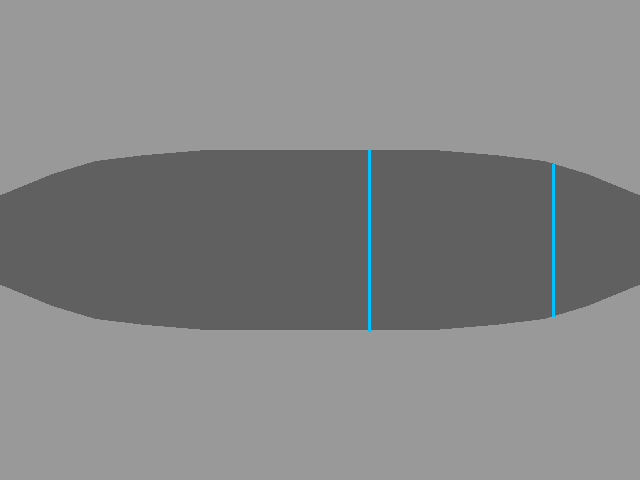
Let’s first think about what our ray hits tell us. We know that a ray is casted per column of pixels on the projection plane. So for each ray, it would seem, we render a column of pixels or something, right? The answer is yes, and I think a graphic would do us wonders here:
So essentially, this graphic details the relationship between our 2D and 3D representations of the world.
The red circle is of course the player. The light blue triangle is the player’s field of view. The deep blue line is an example ray. In the bottom half of the graphic, I show what that ray renders in the 3D world. Essentially, each ray is responsible for rendering a single line of pixels. That’s what the single blue column in the bottom half of the graphic is: the column of pixels that ray renders.
Now that we know what each ray is going to render, let’s figure out how that’s going to happen. First, we are going to need to know the distance between the player and where the ray hit:
One way that we can compute the distance with the Pythagorean Theorem. We know that the distance between the hit and the player is:
hit_dist = sqrt((player.x - hit.x)^2 + (player.y - hit.y)^2)
Where hit is either c_v or c_h depending on which one was closer to the player. Now, we can apply Soh Cah Toa to find this distance much more efficiently. However, I found that at angles 0, 90, 180, 270, etc, there were strange visual artifacts which we’re solved by simply using this.
Let’s review real quick: we know where the ray hit, and we know its distance. We just need to use this to render. This article by Permadi does a great job detailing how we use what we’ve computed to do the rendering. However, I will try my best to explain the same in my own words.
Our goal is of course to render the world onto our screen. And as I have detailed before, our screen is in fact our projection plane. Recall that the projection plane is about 277 pixels away from the player. So essentially, we need to project the part of the world we want to render onto our screen (hence the name projection plane). Let’s assume our ray hit a wall, and we’ve compute the distance. The graphic below details the relationship between our ray, our projection plane, and our player:
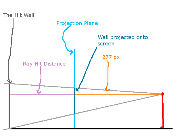
We can actually relate these values with the following equation:
projected wall height / distance from player to projection plane = actual wall height / ray hit distance
With our numbers plugged in, this would be:
projected wall height / 277 = 64 / ray hit distance
And thus, the size of the line of pixels we want to render on our screen is:
projected wall height = (64 / ray hit distance) * 277
And the cool thing is the 64 / 277 part can be precomputed, since these are just constants. But this equation details how we transform the world into “screen space” so to speak.
Correcting for Fish Lense
We are almost done at this point, but there is something I wanted to detail before calling it a day. Recall how we computed the distance between the player and the ray hit. Think about that equation in the context of this image:
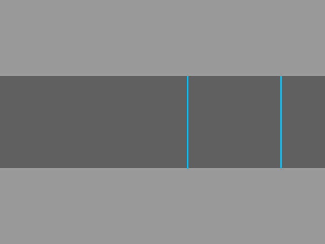
In this case, I show two different rays. If you think about it, these two rays will have a significantly different distance to the player. So using our current ray hit distance, which is just the Pythagorean distance, will give us a world that might look like this:
Now, if we were doing a GoPro Simulator, this might be an ideal effect. For most things however, this is subpar. We call this effect the “Fisheye Effect”. And it comes from using just the straight pythagorean distance. Ideally, we want something more like:
The “corrected distance” is:
hit_dist * cos(theta)
Where theta is the ray angle, not alpha. Visually it comes from this:
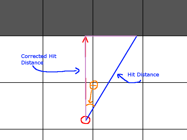
In this case, we apply Cah: That is:
Cos(theta) = corrected_distance / hit_distance
And thus:
corrected_distance = Cos(theta) * hit_distance
Summary
And there we have it! All of the math, minus some implementation specific details. I hope you enjoyed that and learned something. For a more complete picture of this system, please checkout the following links: